The Chain Rule is one of the 4 or 5 main derivative rules that allow you to break down a function into smaller functions in order to find that function’s derivative. As with the other 4 or 5 main derivative rules, the Chain Rule is only applicable under certain conditions. Unlike the other derivative rules, it can be a little difficult to understand and recognize when you can actually use it. If you notice, the phrasing is “can” use it. Remember, don’t think of these derivative rules as things you HAVE TO USE to solve a problem, but rather as tools that can be useful for solving a problem that you may or may not use depending on the details of the problem and what you feel is the best way to approach it.
When Can You Use the Chain Rule?
You “can” use the chain rule (but may not “have to”) when the function you are tasked with taking the derivative of “can be thought of” as (again, don’t think of it as “it is this”; think of it as “it can be thought of as this” since some functions can be thought of as being constructed multiple ways) a function with a function inside of it. What does this mean? Well remember, a function is just some rule that maps inputs (the totality of all possible inputs for a function is called that function’s Domain; this input variable is typically going to be x, but it doesn’t have to be) to outputs (the totality of all possible outputs of a function is called that function’s Range; this output variable is typically going to be y, but it doesn’t have to be). In a calculus class, the Domain of a function will usually consist of a continuous interval of input values (examples of this would be something like All Real Numbers, or x can be any real number from 2 to 100), and the Range of the function will usually consist of a continuous or piece-wise continuous interval of output values. This relationship is usually written as a mathematical expression:
This mathematical relationship is what maps the inputs to the outputs. If you want to know what a number in the domain produces in the function’s range, or set of output values, all you need to do is “plug it in” (I prefer to use the word “substitute”, but to each, their own) to the mathematical expression that defines the function. As the mathematical equation specifies, f(x) is equal to that. This mathematical expression is like a machine that transforms the input number (or expression, as we’ll see later) into an output number (or expression, as we’ll see later). For example, using the previously defined function, let’s determine what the function value is for the input value of 2:
Notice the notation here. f(2) means “the function value when the input is 2”. If you notice, all we did here was replace or substitute all of the original input with the new input. Think of the original function with x as a blank template just showing you the steps you do for any value of x. Don’t like the variable x? Experiment around and put different placeholders. Whatever floats your boat. It’s just a variable. For example, another way to write the original function is:
Or
These all mean the same thing, because they all are telling you to do the same thing. This is an important thing to remember when you are taking a calculus class or any other advanced math class. Things that don’t look the exact same thing written down or described may be the exact same thing as far as we’re concerned because they are mathematically equivalent. In other words, they mean the exact same thing mathematically. So be on the lookout for and practice being able to recognize functions or theorems or problems that look different but are really mathematically equivalent to one another. So nothing too difficult yet, right? Where does the chain rule come into all this?
Now we will take it one step further. Remember, the chain rule can be used to differentiate (take the derivative of) a function that can be thought of as smaller functions that have been put inside one another (these are called composite functions). Let’s look at how these are formed. To form a composite function, you don’t put a single number into a function like we did before, you put in an entire other function. For example, let’s take the original function we had before and introduce a new one as well:
Let’s find f(g(x)). What does this even mean? It looks pretty weird. Well, if you know how to find f(2), or f(3), or f( whatever ), you know how to find f(g(x)). Just replace the original variable in f(x) with g(x), just like the symbols f(g(x)) indicates and just like we did before with all the other substitutions into the original function:
Therefore:
And:
This is just what some people would consider a slightly more complicated version of what we’ve already done, but someone who can see through the clutter and really cut to the heart of what these ideas mean would see it as no different than substituting in a single number. So to get to the burning question of when you can use the chain rule, the answer is whenever you have a function that you can visualize as a composite function (a function within a function). This new function that we created f(g(x)) is an example of a composite function. But this is where it gets a little more difficult. When using the chain rule, you need to recognize when a big function is composed of two smaller functions where one has been put inside the other. This is where some students get tripped up because this can require a little bit of imagination. You have to take on the role of a detective investigating a crime scene. The detective wasn’t there when the crime took place, so he/she didn’t observe exactly what happened. Instead, they need to see the results of what happened and determine what series of events could have caused that end result. We are in this same situation when determining if the chain rule can be used. However, we have one big advantage over the situation the detective finds themself in. The detective can never really know with 100% certainty if their reconstruction of events is correct. We can be 100% certain of whether our conclusion of how a function is a composite function is correct or not by testing it. So in a chain rule type problem, you’ll be given this:
And you’ll need to be able to look at it and determine two different things:
That this is potentially composed of two simpler functions where one has been put inside of another
What those two functions are exactly (one inner function, and one outer function)
In the example we just created, if we think of it as ourselves being the detective trying to recreate the series of events that created the crime scene or the function h(x), it’s pretty easy because we were also the criminal that created the crime scene. Remember, we ourselves put g(x) = 1/x inside of f(x) = x^2 – 2x + 1. But if we hadn’t created the function h(x) ourselves, what clues are there that this can be thought of as a composite function and what those functions could be? You can focus on grouping symbols like parentheses and brackets. So in this function, we see the same function inside a bunch of parentheses pairs. Let’s think of that as our inside function. Now here’s where we get to actually test our theory. If the inside function is indeed 1/x like we think, then we should be able to determine a function that 1/x can be put inside of to create h(x). Here’s kind of a full-proof way to do that. Let’s assign 1/x to a new variable:
Now we can just replace 1/x with u in the function h(x) to determine what the outer function is:
So here we have our answer. h(x) can be thought of as f(u) = (u)^2 – 2(u) + 1 with g(x) = 1/x put inside of it. Before we continue to finally go through how to use the chain rule and use it in this example, let’s double check our analysis so far. If we’re wrong about what the inner and outer functions are at this point, we will most likely get the final answer wrong no matter how well we actually use the Chain Rule. So how do we test that we are correct so far? Well, let’s remind ourselves of what we are claiming at this point. We are claiming that if you take g(x) and substitute into f(u), the resulting function would be h(x). To determine if that is true or not, let’s do it. Let’s substitute g(x) into f(u) and see what we get:
Is that mathematically equivalent to h(x)? Yes, they are the exact same. Therefore, our current claim is correct. h(x) can be thought of as f(u) with g(x) inside of it. Now that all that is out of the way, we need to do the easy part: just use the chain rule. Here’s what the chain rule says as a mathematical formula:
Oh no, we’re looking at another complicated formula. Let’s break down the meaning of this formula a little bit at a time, and you’ll notice that it’s not quite as complicated as it looks. In plain English, I would describe this formula as saying:
If you are taking the derivative of a function that can be thought of as a function within a function, you can do this by: 1) identifying the inner and outer functions, 2) taking both of their derivatives, and 3) writing your answer as the derivative of the outer function, containing the inner function, times the derivative of the inner function.
Let’s finally take the derivative of h(x) using the chain rule. Keep in mind, we’ve already done the hard part of analyzing the function and seeing it as a function with a function inside of it, determining what those two smaller functions are, and checking to see if our analysis was correct. Now we just take both of the derivatives of these functions (maybe using other derivative rules) and put the result together as the chain rule formula says:
Therefore:
And:
Therefore:
That’s it. That’s all we need. Now we just put the pieces together according to the formula:
Put g(x) inside of f’(u) just like the formula says:
Multiply that by g’(x) just like the formula says:
And we’re finished. We can simplify this if we want, but mathematically, we’re done. So let’s take what we’ve learned and create a set of steps you can use to evaluate a derivative using the chain rule:
Determine if you can see the function as a composite function, that is, a function with a function inside of it. This takes some creativity. How do you get good at this? Practice. Practice putting functions inside of functions and looking for patterns of common forms that appear. How do you become good at writing? Maybe start by reading. Read a lot and start to analyze what makes good writing good writing.
If you can see the function as a function inside of a function, great. You just need to determine what those functions are. As we discussed before, if you can identify what you think the inside function is, you can replace every instance of that function with some variable (u, for instance) to tease out what the outer function is. If you don’t see the whole function as a function within a function, does that mean the chain rule can’t be applied? Well, literally yes. If you can’t see the function as an inner function and an outer function, you can’t continue. But that doesn’t necessarily mean it can’t be thought of as an inner function and an outer function. Maybe you’re just not looking at it in the best way.
Once you have the two functions, the inner and the outer, you just take both of their derivatives. Keep in mind that to take both of these derivatives, you may need to use other derivative rules including the chain rule again. Once you have those derivatives, you have everything you need. You just need to put the pieces together. How you put them together is as follows:
Now finally, to get back to a point I made near the beginning of the article: don’t think of the chain rule as “has to be” applied, but rather “can be” applied. In the example that we’ve been looking at, I wouldn’t have chosen to take its derivative using the chain rule normally. There is another way to look at it that makes it an easier problem. I’m not going to think of the function h(x) as
I’m going to think of it as something that is mathematically equivalent:
Here I just multiplied everything out. Now I see something that makes this problem easier. It’s just a bunch of constants and powers of x multiplied and added together. We can use the sum and difference rule, constant multiple rule, and power rule only. No Chain Rule required.
But wait. That doesn’t look like what we had when we solved this problem using the chain rule. What went wrong? Nothing. Remember, we don’t care if things look the same, necessarily. We care if they are mathematically equivalent. And our two solutions are, in this case.
They’re the exact same. If they weren’t, something would have gone wrong. Either we performed the derivative rules incorrectly, or we applied them when they didn’t actually apply. So remember, just because you can do something doesn’t mean you should. Be on the lookout for solving problems the simplest, easiest way possible. That’s how you’ll want to do it on a test. For homeworks and practice, it actually may be beneficial to challenge yourself to solve problems in unnecessarily complicated ways. That can further help you understand the inner workings of how these ideas and theorems work and go together, help you practice your mathematical creativity of seeing complicated things where you would normally see simple things and vice versa, and it will definitely help you appreciate the more efficient ways of doing things. Clean an entire kitchen with just a toothbrush just one time, and you’ll really learn to appreciate the more efficient tools for the job.
The Binomial Probability Distribution is a type of probability distribution that can be described by a probability mass function. Remember that a probability mass function describes the probability of discrete random variables. Therefore, a variable that can be described by the Binomial Probability Distribution is a discrete random variable. This means that it can only take on discrete values (like heads or tails on a coin or the outcomes 1, 2, 3, 4, 5, or 6 on a roll of a die) rather than continuous values (like the length of a table leg produced in a factory which can take on any value across a range of potential values, even decimals like 23.125444234 inches). The Binomial Distribution itself and its corresponding probability mass function are used to calculate the probability of a certain number of successes happening within a certain number of repeated trials of an experiment. Some examples where the Binomial Distribution would be appropriate include:
If you flip a coin 50 times, what is the probability that you would get 12 heads (you need to interpret this as “what is the probability that you would get EXACTLY 12 heads”)?
In a large population of people (millions of people), the prevalence of a disease is 5%. What is the probability that in a random sample of 100 people, 10 people would have the disease (you need to interpret this as “what is the probability that EXACTLY 10 people would have the disease”)?
You work for an airline. You know from previous data that approximately 1/500 people who buy a ticket don’t end up using their plane ticket due to illness or being late and missing the flight. For a flight containing 100 seats, you sell 102 tickets. What is the probability that you have to kick at least 1 person off the flight?
What makes all of these questions or situations solvable using the Binomial Distribution? There are a few qualities. Number one, we are interested in finding the probability that a number of “successes” occur within a number of repetitions of experimental “trials”. In the coin flip example, a head could be considered a success (we are interested in the probability of 12 heads), and the coin flips themselves would be considered repeated trials (we flip the coin a total of 50 times).
Number two, the outcomes of each of the trials is dichotomous, meaning each trial results in a success or a failure (one of only two possible outcomes). In the disease problem mentioned in the previous paragraph, the individual trials would be each person selected. What are the two possible outcomes for each person? They either have the disease (a success) or they don’t (a failure).
Number three, the trials must be independent and identically distributed. What does this mean? Well, independent means that the results of one trial don’t affect the probability of the outcomes of any other trial. A good example of this is the coin flip example. If I flip a coin one time (let’s say the first time of the 50 in the problem above) and it ends up heads, does the probability that the next flip of the coin will be heads change from what I thought it would be before I realized the first flip was heads? It shouldn’t, because once I pick up the coin and flip it again, the fact that it was heads already wouldn’t affect the probability that the next flip will be heads or tails. Once you flip it the second time, the probability just resets.
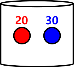
Another example where the trials would be independent would be sampling with replacement. Let’s say you have a box that contains 20 red marbles and 30 blue marbles.
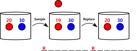
Now before I select the first marble blindly from the box, the probability that I will select a red marble is 20/50, and the probability that I will select a blue marble is 30/50. Let’s say that I mix up the marbles and select one blindly, and when I look at it, it’s one of the red marbles. From this point, I can do one of two things. I can write down that I picked a red marble, place it back in the box, reshuffle everything and pick a new marble.
Now what’s the probability that the next marble is red? It’s back to 20/50 because I put the red marble that I pulled out first back into the box so that there are 20 red marbles out of 50 total marbles. These trials (pulling a marble from the box) are independent because knowing that the first marble is red doesn’t affect the probability that the next one will be red (or blue, for that matter). Once I put the red marble back and remixed the marbles in the box, the probability is back to what it was originally.
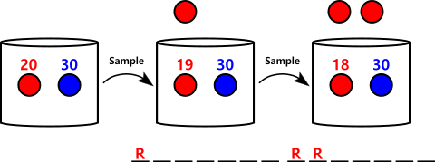
However, what if I don’t replace the marble? If I draw a marble and keep it out of the box, and then draw another marble, does knowing the color of the first marble affect the probability of drawing a certain color on the second draw? Absolutely. Let’s see why.
If I drew a red marble on the first draw and left it out, what’s the probability that the next draw will also be red? It’s not 20/50 anymore because there aren’t 20 red marbles to pick, and there aren’t 50 marbles to pick from. There are only 19 red marbles and 49 total marbles. So if the first marble picked is red, the probability the second one is red is 19/49. But if the first marble is blue, the probability that the second marble is red is not 19/49. If you pick a blue marble first and leave it out of the box for the second draw, you still have 20 red marbles because you haven’t picked one yet, but you still have one marble missing from the original 50. Therefore, your chances of drawing a red on the second draw knowing you drew a blue on the first draw is now 20/49. Because the results of the first trial affect the probabilities of the outcomes in the second trial, these trials are not independent when we sample or draw marbles without replacement. For the Binomial Distribution to be applied, the individual trials MUST BE INDEPENDENT OF ONE ANOTHER!
But what does it mean for the trials to be identically distributed? That just means that the probabilities of the outcomes for each of the trials is the exact same. Here’s an example of a series of trials where the probabilities of the outcomes are not all the same. Let’s say that you have a six-sided die that has one of the faces of the die with a picture of a coin’s head, and the other 5 faces of the die have a picture of a coin’s tails. So when you roll this die, you don’t get a number 1-6. Instead, you get either a head or a tail. Now let’s say that I want to know the probability of getting 4 heads when I flip a coin 7 times, roll this special die 1 time, and then flip the coin another 2 times. This would be 10 trials: 9 by flipping a coin, and 1 by rolling the die with head or tails outcomes.
These trials are all independent. The flips of the coin don’t affect each other, and they don’t affect the outcome of the six-sided die. Likewise, the results of the six-sided die don’t affect the coin flips. Sounds good, right? It does, however, these trials are not identically distributed. The trials involving the coin are, but the single trial (the 8th one) where I’ve decided to determine heads or tails by rolling the die changes the distribution of the outcomes in that trial. The probability of heads is no longer ½ like it was in the coin trials. It’s ⅙ for the die. Therefore, even though the trials are independent (knowing the result of one trial doesn’t change the probability of any other trial), they are not identically distributed. Therefore, this situation couldn’t be modeled by the Binomial Distribution.
So to summarize, the conditions that must be met to model a variable with the Binomial Distribution are:
Repeated trials of an experiment where the outcomes of each trial are dichotomous: success or failure. If there are three or more possible outcomes from a trial, it can’t be modeled by a Binomial Distribution.
The trials themselves are independent and identically distributed. If the results of one trial change the probabilities of the outcomes in a different trial, they are not independent. If the probability distribution for the outcomes are not all the same for each trial, they are not all identically distributed. If either of these things (independence and identical distributions) are not satisfied, it can’t be modeled by a Binomial Distribution.
You are interested in finding the probability of a certain “x” number of successes within “n” number of trials that meet the above criteria – trials that meet this criteria are called Bernoulli trials.
What Math Defines the Binomial Probability Distribution Mass Function?
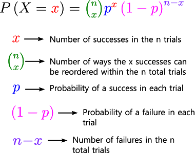
The probability mass function (the function that reports out the probability associated with a value of the variable) is:
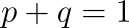
So to determine the probability that X takes on a specific value in a process that can be modeled with a Binomial Distribution, you just substitute the value of X in for x in the function and the number you get out is the probability that X is that value in the Binomial process. Now all of these numbers parameters actually mean something. Let’s review some interesting properties of the Binomial Distribution that arise because the results of the individual trials are dichotomous. First of all, the number of successes and failures must add up to the total number of trials. Why? Because those are the only two things that can happen. So if I tell you there were x successes in n trials, then how many failures were there? Let’s do a little bit of math. We know:
Therefore,
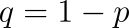
And as you can see, the number of failures is the number of total trials minus the number of successes. This is because the sum of the successes and failures must add to the total number of trials. What else comes about in the math because of the dichotomous nature of the individual trials? The probability of a failure is one minus the probability of a success. Let’s see why by looking at the details of a single trial and remembering what we know about basic probability theory. We know in each individual trial that there are only two possible outcomes: success or failure. We also know that these are individual discrete outcomes, meaning the chances of them both happening (probability of any individual trial having a success AND a failure) is zero. Therefore, we know that we could add their individual probabilities to equal to the total probability of 1.
We can rearrange this algebraically to see that the probability of a failure is one minus the probability of a success:
So the probabilities raised to their powers in the binomial probability mass function just represent the probabilities of successes and failures raised to the power of the number of times a success or failure appears in the trials and then multiplied together. We’ll see in a little bit where that comes from.
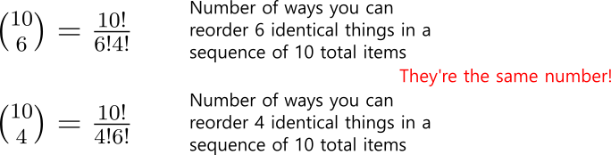
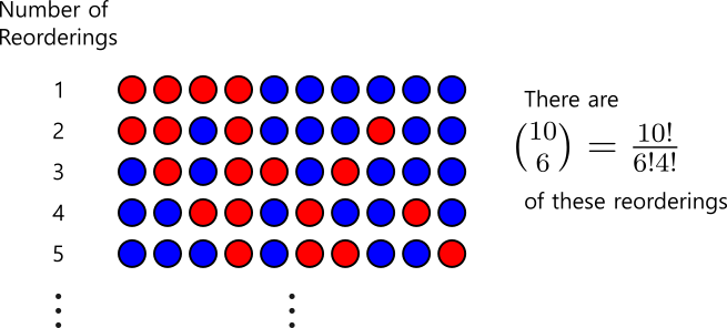
But what about that big coefficient at the beginning. That is called a Combination. You can read it as “combinations of n taken x at a time” or “n choose x”. This can be interpreted two ways (and probably more). “n choose x” is the number of ways that you can take “n” number of things and group them into a group of size “x”. Another way to think of this number (which is the way that we’ll want to interpret it for it to make sense in the context of the binomial distribution) is “n choose x” represents the number of reorderings of “x” identical items in a sequence of “n” total things. Let’s discuss what this really means with an example. If I have 10 total marbles in a sequence that consist of 4 red marbles and, therefore, 6 blue marbles, and we want to know how many different reorderings of these marbles we can have, we would calculate 10 choose 4. You’ll also notice that we could have approached it as the number of ways the 6 blue marbles can be reordered within the 10 total spaces in the sequence. That would be 10 choose 6. If you look at the math, 10 choose 4 and 10 choose 6 are the exact same calculation. They result in the same number.
10 choose 4 calculation and 10 choose 6 calculation
So in our Binomial probability mass function, the coefficient in the beginning is a calculation of how many ways our “x” successes can be rearranged or reordered inside the sequence of “n” total trials. As you’ll see later, that is an important thing to consider when determining the probability of “x” number of successes within “n” sequential Bernoulli trials. So now that we see how all the individual numbers (and groups of numbers) in the Binomial distribution probability mass function actually have a direct meaning, let’s look at how to use the probability mass function to answer some questions.
Using the Binomial Probability Mass Function to Solve Problems
So now let’s look at some problems and how they can be modeled by a Binomial distribution, and we can use the Binomial probability mass function to find the probabilities of different situations. Let’s go back to a similar situation that we saw near the beginning.
If you flip a coin 10 times, what is the probability that you would get 8 heads?
Now first, let’s look at how the details of the Binomial distribution arise naturally from the situation described in this problem. First of all, we have 10 repeated trials. Those can be represented by the 10 blanks below
10 blank trials picture
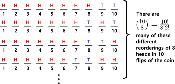
An “H” in a blank means that toss of the coin resulted in a head and a “T” in a blank means that toss of the coin resulted in a tails. So let’s look at one result where we have 8 heads in the 10 total flips of the coin.
Let’s calculate this probability. I’ll let Hi represent the ith toss is a heads, and Tj represents the jth toss results in a tails. So that first result could be denoted as:
Probability notation for probability of first 8 heads
Notice if we only have 8 heads, there HAVE TO BE 2 tails. That’s why in that probability statement the last two are indicated as tails. That has to be true. If those are not accounted for, we are not finding the probability we want. If we look at each of these events (H1, H2, H3, etc.) they are all independent of each other. The fact that the first toss of the coin is heads doesn’t change the probability that the second will be heads from what the probability was before or the third and so on. Also, the distributions of the individual trials are all identical. They’re all 50% probability heads and 50% probability tails. Remember, for independent events, to find the probability of their intersection (their AND probability), you just multiply the separate probabilities together. So the probability of our specific sequence of heads and tails can be calculated as:
Formula — probability of intersection is individual probs multiplied
So is this our answer? No. This would be the answer if the question was “what is the probability that the FIRST 8 tosses of the coin are heads?”. We’re trying to answer the question about the probability of there being 8 heads ANYWHERE in the 10 total tosses. We don’t care if they’re the first eight, the last eight, or if the eight heads are dispersed any other way around the 10 total flips of the coin. So what do we need to do? We need to consider how many different ways these 8 heads can exist or be reordered within the 10 total tosses. That’s where that “n choose x” comes into play. If we calculate 10 choose 8 (or 10 choose 2, remember they’re actually the same calculation), that would be how many different sequences of heads and tails exist with 10 total tosses and 8 heads. Because all of the trials are identically distributed, any sequence of 8 heads in the 10 total tosses would have the same probability. That’s why we multiply the probability by this “n choose x” factor.
Once we multiply those together, we now know the total probability of getting 8 heads IN ANY ORDER when we toss the coin 10 total times. And that is what we’re looking for in this problem. Not the probability that we get 8 heads in a SPECIFIC order, but in ANY order. That’s why we have to multiply that probability by “10 choose 8”. The “10 choose 8” accounts for all the possible orders of the 8 heads within the 10 coin tosses.
So this is how to solve a classic, textbook binomial distribution problem. If you can understand this coin flip problem, you can apply the exact same logic to any other binomial distribution problem. You just have to make sure that each of the repeated trials are dichotomous (only two outcomes), independent, and identically distributed. Then, if you are interested in finding the probability of x number of successes in n total outcomes IN ANY ORDER, you can apply the binomial probability mass function to answer that question no matter the other details of the problem. To see this, let’s consider a more complicated problem that may not immediately look like it can be modeled by a binomial distribution:
You work for an airline. You know from previous data that approximately 1/500 people who buy a ticket don’t end up using their plane ticket due to illness or being late and missing the flight. For a flight containing 100 seats, you sell 102 tickets. What is the probability that you have to kick at least 1 person off the flight?
First, let’s discuss how this can be thought of just like the coin flipping problem. In the coin flipping problem, we had 10 repeated trials. Each toss of the coin was a separate trial. What are the trials in this example? Each person that does or doesn’t show up for the flight is a trial. In the coin toss example, each trial had two possible outcomes only: heads and tails. Is that true for the trials in this airline problem? Yes, the two possible outcomes for each trial or person is one of two: they are present for the flight, or they are not present for the fight.
Are the trials independent? This is where it gets a little hairy. In real life, probably not. Let’s see why. Some people travel in groups. So let’s consider that there’s a family in these 102 people that bought a ticket: a husband, a wife, and 2 kids. If you know the result of the “husband trial”, meaning that you know whether the husband is present or not present for the flight, does that change the probabilities of the wife and 2 kids being present for the flight? I would say yes. Knowing that the result of the “husband trial” is success, that should make it much more likely (probably nearly 100%) that the wife and kids are present as well. If the result of the “husband trial” is failure, that should make it much less likely (maybe nearly 0%) that the wife and kids trials will be a success. So in real-world situations, we’d actually need to consider that. And if that is happening (we have families traveling, or groups, or people from the same business conference, etc.) knowing one person has missed the flight may make it more or less likely that other people will miss the flight. In this situation we’re trying to solve, we are going to assume that is NOT TRUE. We are going to treat these ticket holders like they are completely independent of one another. Therefore, the trials will be independent.
In the coin toss example, the trials were identically distributed. That meant every toss of the coin had a 0.5 probability of heads, and 0.5 probability of tails. Do all the trials in the airline example have identical distributions? It depends on the information you have available. If you know one of the people who bought a ticket has a connecting flight that is scheduled to get in with just enough time to run across the airport and board this flight, that would make it less likely than an average person that they will make the flight. If you know one of the people who bought a ticket is staying in a hotel right by the airport, they are catching this flight for an important business thing, and they have one of those fast pass things that lets them go through the checkpoints really quickly, that would make it more likely than the average person that they would make their flight. Because we don’t know any of this, we treat them all like they’re the same. Therefore, when the problem says 1/500 people miss their flight, we use that probability for each individual person and say each individual person (without knowing any better) will have a 1/500 chance of missing their flight. For that reason, we can treat the trials as identically distributed: 1/500 probability of a trial resulting in missing the flight, and 1-1/500 or 499/500 probability of a trial making the flight. So all the conditions are met for this situation to be modeled as a Binomial Probability Distribution.
Now we just need to make sure the question we’re trying to answer has to do with finding the probability of a certain number of successes IN ANY ORDER within a certain number of trials. That is true in this case. Let’s discuss why. The real question is “What is the probability that you have to kick at least 1 person off the flight?”. That doesn’t sound like the question we had with the coin tosses, but it actually is. Let’s think for a second. Kicking a person from the flight would mean that more people showed up for the flight than there are seats. So what we really need to interpret this as asking is “What’s the probability that more than 100 people show up for the flight?” If 100 or fewer people show up for the flight, we don’t have to kick anyone from the flight. If EXACTLY 101 people show up for the flight, we have to kick 1 person. If EXACTLY 102 people show up for the flight, we have to kick 2 people from the flight. And we should agree that more than 102 people can’t show up, because it says we only sold 102 total tickets. So that’s how this becomes a probability question we can answer. What is the probability that EXACTLY 101 OR EXACTLY 102 people show up for the flight out of the 102 total number of people that could show up for the flight. Be aware that the total number of trials is not the number of seats (100), it’s the number of ticket holders (102) because we’re trying to figure the probability that a certain number of those 102 ticket holders are successes (showing up for the flight).
Now because we are trying to find the probability of EXACTLY 101 OR EXACTLY 102 successes, we can find the probability of EXACTLY 101 and EXACTLY 102 successes separately and just add them together to find their OR probability. Why? Because they are mutually exclusive. If you know EXACTLY 101 people showed up for the flight, what’s the probability that EXACTLY 102 people showed up for the flight (or EXACTLY 100, or EXACTLY 99, or EXACTLY 98, etc.)? It’s now zero. If I know EXACTLY 101 people showed up, the probability that also EXACTLY 102 people showed up is zero. This means the probability that EXACTLY 101 AND EXACTLY 102 people show up for the flight is zero, meaning they are mutually exclusive events. For mutually exclusive events, you can add their individual probabilities to find their OR probability. So in this problem, we just need to find two separate probabilities and add them together to answer the question. And since we’ve discussed that we’re assuming all the conditions are met for this situation to be modeled by a Binomial Distribution, we can use the Binomial Distribution Probability Mass function to find those probabilities:
And so the end result is:
Final answer
So What’s the Bottom Line?
The bottom line is that any time you have repeated trials of an experiment that only ever have two possible outcomes (success or failure), and the trials don’t affect each other (independence), and the distributions of the outcomes are all identical (the probability of a success or failure is the same in each individual trial), the probability of x number of successes within the n trials can be modeled by the Binomial Probability Distribution. This assumes that the order of the successes in the sequence does not matter. So if we look at the airline example again, and we say “what is the probability that you’ll have to kick the passenger in seat 3A off or the passenger in seat 6B off the plane?”, we can’t model it as a strictly binomial distribution anymore. We are still talking about a similar situation, but now we’re talking about specific passengers (meaning specific trials in the sequence of trials) and we therefore can’t multiply by the “n choose x” coefficient at the beginning which would cause us to find the probability of kicking off any two passengers, not the specific ones we’re talking about in those specific seats. And we also saw how the numbers in the probability mass function actually mean something. The coefficient at the beginning accounts for the number of possible ways you can have that many successes within that many total trials. The probabilities raised to their respective powers representing the number of successes and failures multiplied together calculates the probability of a single sequence of trials that has that many number of successes within the total. So when you multiply the probability of one sequence of x successes within n total trials times the number of different ways you can actually get x successes within n total trials, you get the total probability of x number of successes in any order within the n total trials.
And as we saw, if the problem is really asking to find the probability that a few different numbers of successes happen (at most 3, meaning 0, 1, 2, or 3; at least 10, meaning 10, 11, 12, etc.; more than 10, meaning 11, 12, 13, etc.), you can just find the probability of each specific number of successes using the binomial distribution mass function and add them together to find their OR probability (any of those number of successes happen).