Tag: artificial-intelligence

  • Hypothesis Testing Part 3: Bringing it All Together

    So now that we know what sampling distributions are, we can better understand the mathematical ideas behind hypothesis testing. The basics of hypothesis testing is you want to prove something about the population (a population parameter) by assuming something about it, and seeing if you get sample data that is unlikely based on that original assumption. If you can calculate that the sample data that you actually have is unlikely assuming what you have assumed is true in the population, then you can say that what you’ve assumed is true in the population is not likely to be true. This assumption about the population is called the null hypothesis. The good news is that now that we know a lot about sampling distributions, we can calculate the probability of getting sample data with certain sample statistics based on population parameters. Let’s look at this in more detail.

    Hypothesis Test on a Population’s Mean

    One application of hypothesis testing is coming to a conclusion as to whether or not a population’s mean is a certain value. So let’s look at a scenario. Let’s say you work as a biologist and the long standing knowledge in the field is that the average length of this species of frog is 5 inches. Based on your experience in the field studying these frogs, you think that they are longer, on average, than 5 inches. How do you challenge the long standing claim of an average length of 5 inches? This is a perfect situation for hypothesis testing. If we are able to gather enough evidence that would be very unlikely to exist assuming that the assertion of the null hypothesis is true, we can conclude that the assertion of the null hypothesis is not true. So let’s look at how this will play out.

    First, we identify our null and alternative hypotheses. The null hypothesis is the established truth that you are hoping to find evidence against. The alternative hypothesis is what you’re trying to find evidence to support, because you think it is true in reality. So for this situation with the average lengths of frogs, our hypotheses would be:

    H0:μ=5H_0: \quad \mu=5
    H1:μ≠5H_1: \quad \mu \neq 5

    Basically, we’re assuming that the null hypothesis is true the whole time. So the next step would be to gather evidence. How do we gather evidence in this situation? It comes from sample data. So we would gather a sample of frogs and measure the average length of frogs in that sample. In this sample, we need to make sure that we satisfy the conditions needed to use the details of the sampling distribution of sample means. Remember, these conditions are: the sample needs to be a simple random sample, the sample size can’t be 10% or more of the population size, and the distribution of frog lengths in the population either needs to be normally distributed or the sample size must be at least 30 so that the central limit theorem can be applied for normality of sample means. Let’s say that we took a sample with these qualities, and these are the summary statistics:

    x‾=5\bar{x} = 5
    s=1.1s = 1.1
    n=40n = 40

    So let’s look at these sample statistics in a little bit of detail. As you can see, we took a simple random sample of 40 frogs, and the average height of those 40 frogs was 6 inches. Does this provide evidence that you’re right? That the true average height of all frogs in the population is more than 5 inches? Yes. If you’re thinking that this provides good evidence that the true mean of frog lengths is more than 5 inches because you think to yourself, “we have a sample of 40 frogs whose mean is 6 inches. That would probably be unlikely to happen if the true mean in the population was only 5 inches. That’s why this is strong evidence that the true mean length of frogs in the population is more than 5 inches”, then you’re thinking like a statistician. That’s the exact logic that we’re going to use here. However, the issue with that logic is the phrasing, “that would probably be unlikely if the population mean was only 5 inches”. And that’s the whole issue with this data. Is a sample mean of 6 inches from a sample of size of 40 really that unlikely if the true mean is only 5 inches?

    First, let’s realize that it is theoretically possible to get a sample of 40 frogs with a mean length of 6 inches. When we say that we are assuming the true mean length of the population of frogs is 5 inches in the null hypothesis, we are not saying that they are all 5 inches. If the population mean is 5 inches, some of the frogs will be longer than that. Some will be shorter than that. Is it possible that we got a simple random sample, and just due to random chance, we happened to get a sample of 40 that were longer than average? In other words, is it still possible that the population of frogs has a mean length of 5 inches, but we still get a sample of 40 frogs with a mean length of 6 inches? Yes, it’s definitely possible that happened.

    So now that we can agree that this sample is possible to occur even if the true mean length of frogs in the population is as low as 5 inches, you may counter with, “So it is possible that this could happen, but it would be very unlikely. I would think that if you take a sample of 40 things, the average of those 40 would be closer to the true average. So if the true mean of lengths in the population is only 5 inches, we should have gotten a sample of 40 with a sample mean very close to 5. Since 6 is not very close to 5, we can still say that this is very unlikely.” Well, there’s a flaw in this reasoning as well. You are claiming that 6 is too far away from 5 without directly considering the parameter that determines the far-ness of random variables from the mean. I’m of course referring to the standard deviation. If you claim that 6 is very far away from 5, maybe it is and maybe it isn’t. It all depends on the standard deviation of the distribution. If the standard deviation of the lengths of frogs is large, then it is more likely that you get lengths that are further from the mean. So what counts as far from the mean is really the number of standard deviations the value is from the mean. This idea should sound familiar. It’s called a z-score. So in other words, you can’t make a claim that 6 inches is too far away from the expected value of 5 inches without taking into consideration the inherent variability of the population distribution.

    So if we go back to what we learned in the previous post about sampling distributions, we can actually tie this all together and not just do some hand-waving explanation of what is likely or unlikely. We can instead calculate the likelihood of the sample data looking as severe as it does (or even worse) based on the assumption of the true population mean using the details of the sampling distribution of means.

    Remember from the previous discussion that the sampling distribution of sample means of a certain size can be approximated with a t-distribution if the true standard deviation of the population is not known. That will normally be the case. So if we only have the sample data, we will use the sample standard deviation as a best approximation to the population standard deviation. Under this condition, the best distribution to use for the sampling distribution of means is the t-distribution. So we just convert our sample mean of 6 into the corresponding t-statistic. We can then calculate the probability that this t-statistic is as far from its mean of 0 or further to the right. This will correspond with the probability that our sample mean is 6 or larger. This is that probability that we keep looking for. And this probability has a name. It’s called a p-value. You can see that if we have a small p-value, that is evidence for the alternative hypothesis since that literally means the probability that you would get a sample with the details that you did or even more extreme assuming the null hypothesis is true. Another way to think of this is that a low p-value means an unexpected result based on the assumption of the null hypothesis. The following figure outlines this whole process and the math involved:
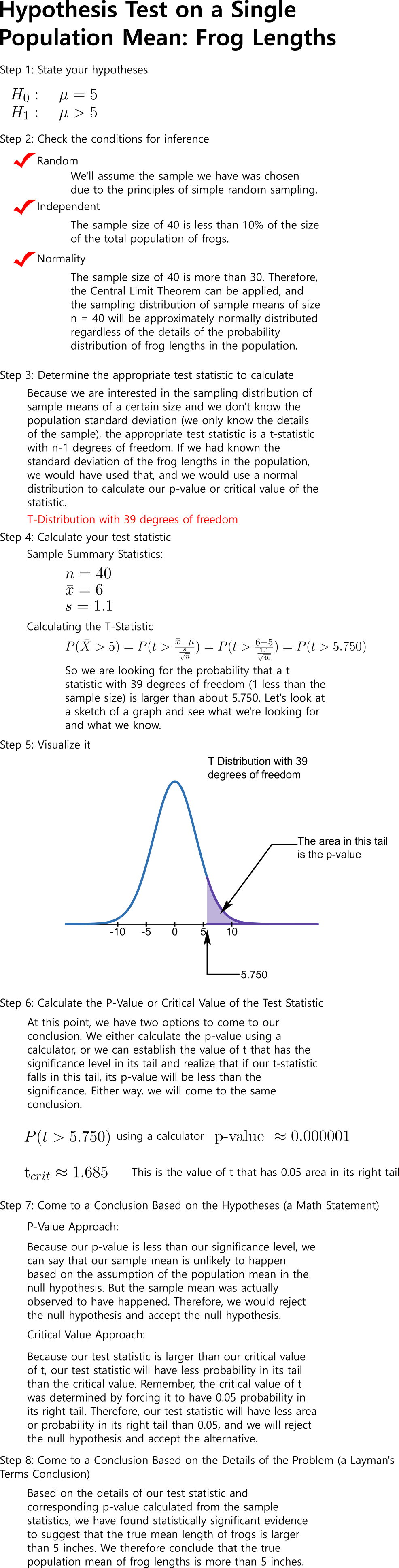
    So as you can see, our intuition was right. It turns out that the probability of getting a sample of size 40 with a mean 6 inches if the population mean of frog lengths was really only 5 inches is incredibly unlikely. How unlikely? That’s what our p-value tells us. But, remember that it depends on the variability of the data which we accounted for in our analysis. So using sampling distributions, we don’t have to guess at how likely or unlikely our data is based on the assumption of the population distribution. We can actually calculate it and therefore defend our conclusion.

    Now this was an extensive discussion for a hypothesis test on a single population’s mean. All other hypothesis tests have the same sets of steps. The details of the conditions that have to be met, the distribution of the test statistic that you use, and some of the other steps may be a little different, but the flow of the logic and how you support you final conclusion are all based on the same idea. If you understand what a hypothesis test is really well one time, you can apply that logic to any other hypothesis test. The videos at the end of this lesson delve into other examples of hypothesis testing.

  • Hypothesis Testing Part 2: Sampling Distributions

    Remember, hypothesis testing works by assuming a value of a population parameter (the null hypothesis) and calculating how likely you are to see your associated sample statistic (or an even more severe value given by your alternative hypothesis) on any given sample. So let’s say we have a sample statistic like a mean or proportion. How do we calculate the likelihood or probability that we would observe a sample statistic this severe or more? It all comes down to the details of the relevant sampling distribution.

    What is a Sampling Distribution?

    A sampling distribution is a type of probability distribution that arises in the situation where you are trying to determine the probability of a sample statistic having a specific value or range of values. So for instance, let’s say we want to answer the question, “What is the probability that any given sample of n from a population has a sample average of x‾\bar{x} or more?” There is a way to figure this out if you know the details of the distribution in the population that the sample comes from, or if certain conditions are met with the sample.

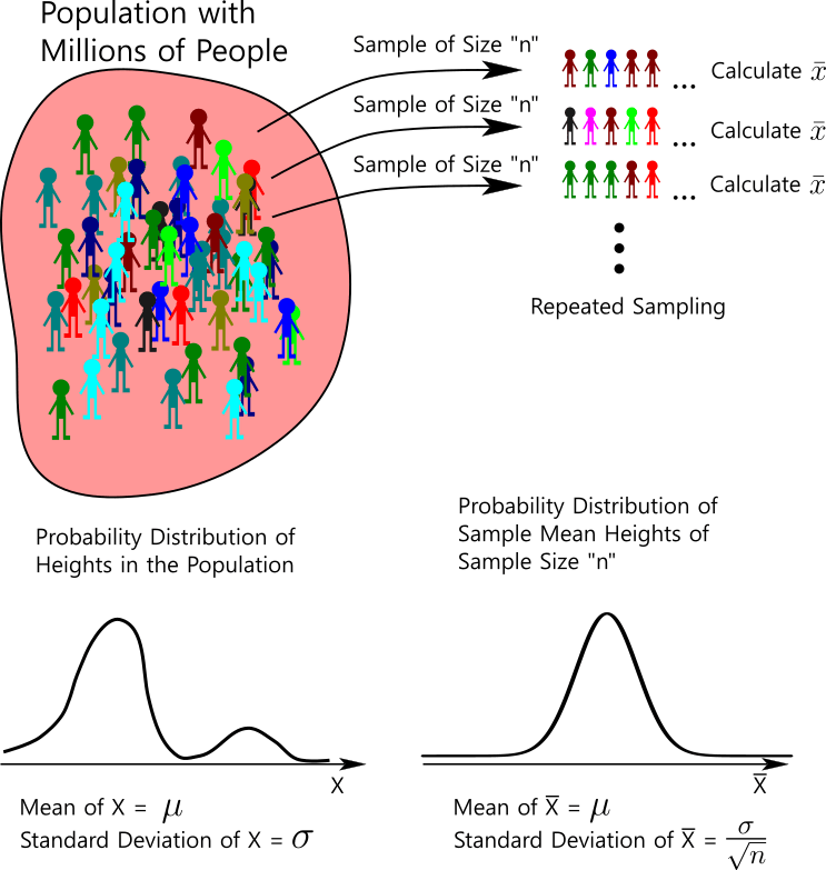
    So let’s focus on a sampling distribution for a specific sample statistic. Let’s start by talking about the sampling distribution for sample means of a certain sample size nn from a population. First of all, let’s understand that a sample mean from a specific population is itself a random variable. If you have a population of people whose heights follow a specific probability distribution, an individual random person’s height is a random variable since it can be various values with a different associated probability for each value. We can call this variable that represents a random person’s height xx. But what about a sample mean from a sample of 40 people? Well that is also a random variable. If you take a simple random sample of 40 people from this population and measure their heights, and find the average height in that sample, is it perfectly predictable? No. But, as we shall see an average of 40 people’s heights from this population is much more predictable than any individual person’s height, meaning it has a much lower variance or standard deviation.

    But what does the distribution of sample means from a sample of size nn look like, and what characteristics does it have (like mean and standard deviation)? It turns out that if certain conditions are met, the probability distribution of sample means of samples of size nn is approximately normal with a mean of μ\mu and a standard deviation of σn\frac{\sigma}{\sqrt{n}} where σ\sigma is the standard deviation of the variable xx in the population distribution of xx. In other words, if we were to take a sample of size nn from a population that has some randomly distributed variable, we can calculate the probability of the sample having a sample mean above some value or between two values by any method you normally use to find the probability that a Normally distributed variable obtains a specific range of values (think of z-scores and normcdf on your calculator and all that jazz).

    Let’s look at the parameters of this sampling distribution of means in a little more detail. The mean of the sample means is the mean of the random variable in the population. So if we had a population of people and the height of a random person can be treated as a continuous random variable, the population has a certain mean height of μ\mu. That is, the average of all the heights in the population is μ\mu. What is the average value of all sample means of a specific sample size nn? It’s also μ\mu. In other words, the mean of the sample means is the mean of the random variable in the population. Another way to phrase this is, “the average of all the averages is the average.” This shouldn’t be a particularly shocking result. What is much more interesting is what the standard deviation ends up being.

    First, let’s discuss what we’d expect. What do you think is more predictable: the height of a single random person from the population, or the average of 50 random persons’ heights from the population? It shouldn’t take too much explaining to see that the average of 50 people would be more predictable. Why? Because rare events start to average out with a bigger sample size. Is it fairly likely to obtain a single person with a weird height? It’s probably not that unlikely. But if you get one weird height (by weird, I mean a height in a low probability interval of heights) out of 50, will that make the average that unpredictable? No, that one weird height will get averaged into the other 49, and as long as you don’t have many weird heights in that one sample, the average will not be that different than the true average in the population. Even two or three weird heights probably wouldn’t change the average of 50 that much from being around the true average. In other words, in samples, the sample average is more predictable than any single random element from the population. This is reflected in the standard deviation of sample means (σx‾\sigma_{\bar{x}}). If the standard deviation of the random variable in the population is σ\sigma, then the standard deviation of the sampling distribution of sample means has a standard deviation of σn\frac{\sigma}{\sqrt{n}}. So if you look at the math, the larger the sample size, the smaller the standard deviation of the sampling distribution of means. And if a random variable has a small standard deviation, then that means the values are, on average, not very far from the mean. Therefore, the values of the variable are more predictable. They are all huddled around the mean.

    So now that we’ve given an example of what a sampling distribution is, we’ll look at the details of some common sampling distributions.

    Sampling Distribution of a Single Population’s Sample Means

    This is what we’ve already been looking at in the previous example. It turns out that if certain conditions are met, the sample mean of a sample of size nn behaves as a random variable, meaning it can take on different values at varying probabilities. The original population distribution and the parameters (like mean and standard deviation) allow us to predict the probabilities of what the various sample means can be. But this predictive power is only true if certain conditions are met. So what are those conditions?

    Condition 1: The sample has to be a simple random sample

    This condition will need to be met for most probability and inferential statistics questions. Basically, in order for the probability distributions we have to mean anything, we can’t introduce any type of bias or change the probabilities in any way. If we do, we can’t use the same probability distributions.

    Condition 2: The sample size cannot be small

    Why can the sample size not be too small? If the sample size is too small, we can’t assume that the sampling distribution of means is normally distributed (or basically predictable in any way). We would only be able to proceed if we knew that the distribution of the original variable in the population follows a normal distribution. If the sample size is not too small, the variable that represents the sample means can not be assumed to be normally distributed. For means, that magic number is 30. If the sample size is at least 30, the central limit theorem shows us that the sample average will follow a normal distribution.

    Condition 3: The sample size cannot be too big

    One of the assumptions built into the math that we are going to use to analyze sampling distributions is that the elements in the sample are independent of one another. This would definitely be true if we were sampling with replacement. However, when sampling, you typically don’t sample with replacement. But if the population is large compared to the sample size, the probabilities are not very different from sampling with replacement. Therefore, the sample elements can be treated as if they were sampled with replacement. The magic number for this condition is 10%. If the sample size is less than 10% of the population size, the probabilities don’t change that much as you sample, and the elements in your sample can be treated as if they were sampled with replacement (independent).

    If these conditions are met, the sampling distribution of means can be modeled as a normal distribution with the following parameters:

    As you’ll see later, one of the main reasons you learn about sampling distributions is to test predictions about population parameters. In those situations, you rarely know the population standard deviation. As you can see in the above formula, you need to know the population standard deviation to determine the sampling distribution standard deviation and then calculate probabilities. When the population standard deviation is not known, you use the next best thing: the sample standard deviation. In the formula above, you just replace the population standard deviation with the sample standard deviation. Then, the distribution of normalized sample means follows a t-distribution with n−1n-1 degrees of freedom.

    Therefore, when the population standard deviation is not known, the normalized sample mean random variable can be modeled as:

    x‾−μxsn∼tn−1\frac{\bar{x}-\mu_x}{\frac{s}{\sqrt{n}}} \sim t_{n-1}

    Sampling Distribution of the Difference of Two Sample Means from Two Different Populations

    Now it turns out that a linear combination of sample means from two (or more for that matter) populations also follows a normal distribution. Where this will show up later in hypothesis tests is when you are interested in the value of the difference between two means between two different populations. So that’s what we will focus on here: the sampling distribution of the difference between two sample means. So what conditions for inference need to be met? The same conditions for a single sample mean, but you have to check it for both samples. If both samples meet those conditions for means that we discussed in the previous paragraphs, then the difference in sample means can be modeled as a Normal Distribution with the following parameters:

    Just like before with the discussion of the sample mean sampling distribution, the standard deviations in the population are rarely known. Therefore, we just replace the standard deviations of the population with the next best thing: the sample standard deviations. Once we do this, the normalized variable follows the t-distribution:

    (x‾1−x‾2)−(μx1−μx2)s12n1+s22n2∼tmin⁡(n1−1,n2−1)\frac{(\bar{x}_1-\bar{x}_2)-(\mu_{x_1}-\mu_{x_2})}{\sqrt{\frac{s_1^2}{n_1}+\frac{s_2^2}{n_2}}} \sim t_{\min(n_1-1,n_2 – 1)}

    Be aware that this notation means the degrees of freedom is the minimum of the two degrees of freedom from the two samples.

    Sampling Distribution of a Single Population’s Sample Proportions

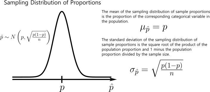
    This distribution arises when you are taking samples of a certain size and you are trying to predict the proportion of observational units within the sample that take on the value of a certain variable. That variable would have to be a binary categorical variable (it’s a categorical variable with either a success or failure level). So it turns out that if certain conditions are met, the sample statistic p_hat can be modeled as a random variable with a probability distribution approximated by a normal distribution. What are those conditions? Well two of the conditions are the same as they were for means. That is, the sample size can not be too big or it will violate the assumption of independent sampling, and the sample must be from random sampling. The last condition is the same as well, in that the sample size can’t be too small. However, what counts as “too small” is different for proportions.

    Condition 2: The sample size cannot be too small

    This number is different because it doesn’t work on the same principle of the Central Limit Theorem which is used for means. For proportions, the sampling distribution of sample proportions can only be modeled by a Normal Distribution because it actually follows a linear transformation of a Binomial Distribution, but a Binomial Distribution can be approximated as a Normal Distribution if the sample size is large enough. This is the golden number that determines if the sample size is large enough for a sampling distribution of sample proportions can be modeled as a Normal Distribution. npnp and n(1−p)n(1-p) have to both be at least 10. So as you can see, you can get away with taking a relatively small sample if the proportions of success and failure of the variable in the population are both relatively big (around 50%). However, if either the probability of success or failure is very small (the other would then be very big), you will need a larger sample size so that those products of sample size and proportions are both at least 10.

    Sampling Distribution of the Difference Between Two Sample Proportions from Two Different Populations

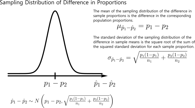
    Just like the sampling distribution of the difference between two sample means is just an extension of the sampling distribution of a single mean, the sampling distribution of a linear combination of two sample proportions is just an extension of the sampling distribution of a single proportion. So all the conditions that must be true for a single sample proportion for its sampling distribution to be approximated with a normal distribution must also be true for both samples when we are determining the sampling distribution of a linear combination of sample proportions. Just like for a linear combination of means, we are most interested in specifically the difference between two population proportions. So that is what we will focus on here. If all the conditions discussed previously for proportions are met for both samples, the difference between to sample proportions can be modeled as a Normal Distribution with the following parameters:

    What’s the Point?

    The point of all of this discussion of sampling distributions is so that we can determine probabilities that sample statistics (means, proportions, or differences of these between two samples) take on certain ranges of values. For instance, if you knew the probability of or the proportion of people in a population who are left-handed, and the conditions for inference of a sample proportion as we discussed earlier are met, we can calculate the probability of getting a sample proportion of left-handed people greater than a certain amount by using the details of the normal distribution that it follows. The following video instructions will make this more clear.

    However, the real point of all of this (as far as you’re concerned in this class) is that we can use these ideas of sampling distributions to indirectly test certain assumptions about the population distribution parameters. This process of testing certain values of population parameters using sample data and corresponding sample statistics and their corresponding sampling distributions is called Hypothesis Testing. We’ll explain how that all works in the next blog post.