So now that we know what sampling distributions are, we can better understand the mathematical ideas behind hypothesis testing. The basics of hypothesis testing is you want to prove something about the population (a population parameter) by assuming something about it, and seeing if you get sample data that is unlikely based on that original assumption. If you can calculate that the sample data that you actually have is unlikely assuming what you have assumed is true in the population, then you can say that what you’ve assumed is true in the population is not likely to be true. This assumption about the population is called the null hypothesis. The good news is that now that we know a lot about sampling distributions, we can calculate the probability of getting sample data with certain sample statistics based on population parameters. Let’s look at this in more detail.
Hypothesis Test on a Population’s Mean
One application of hypothesis testing is coming to a conclusion as to whether or not a population’s mean is a certain value. So let’s look at a scenario. Let’s say you work as a biologist and the long standing knowledge in the field is that the average length of this species of frog is 5 inches. Based on your experience in the field studying these frogs, you think that they are longer, on average, than 5 inches. How do you challenge the long standing claim of an average length of 5 inches? This is a perfect situation for hypothesis testing. If we are able to gather enough evidence that would be very unlikely to exist assuming that the assertion of the null hypothesis is true, we can conclude that the assertion of the null hypothesis is not true. So let’s look at how this will play out.
First, we identify our null and alternative hypotheses. The null hypothesis is the established truth that you are hoping to find evidence against. The alternative hypothesis is what you’re trying to find evidence to support, because you think it is true in reality. So for this situation with the average lengths of frogs, our hypotheses would be:
Basically, we’re assuming that the null hypothesis is true the whole time. So the next step would be to gather evidence. How do we gather evidence in this situation? It comes from sample data. So we would gather a sample of frogs and measure the average length of frogs in that sample. In this sample, we need to make sure that we satisfy the conditions needed to use the details of the sampling distribution of sample means. Remember, these conditions are: the sample needs to be a simple random sample, the sample size can’t be 10% or more of the population size, and the distribution of frog lengths in the population either needs to be normally distributed or the sample size must be at least 30 so that the central limit theorem can be applied for normality of sample means. Let’s say that we took a sample with these qualities, and these are the summary statistics:
So let’s look at these sample statistics in a little bit of detail. As you can see, we took a simple random sample of 40 frogs, and the average height of those 40 frogs was 6 inches. Does this provide evidence that you’re right? That the true average height of all frogs in the population is more than 5 inches? Yes. If you’re thinking that this provides good evidence that the true mean of frog lengths is more than 5 inches because you think to yourself, “we have a sample of 40 frogs whose mean is 6 inches. That would probably be unlikely to happen if the true mean in the population was only 5 inches. That’s why this is strong evidence that the true mean length of frogs in the population is more than 5 inches”, then you’re thinking like a statistician. That’s the exact logic that we’re going to use here. However, the issue with that logic is the phrasing, “that would probably be unlikely if the population mean was only 5 inches”. And that’s the whole issue with this data. Is a sample mean of 6 inches from a sample of size of 40 really that unlikely if the true mean is only 5 inches?
First, let’s realize that it is theoretically possible to get a sample of 40 frogs with a mean length of 6 inches. When we say that we are assuming the true mean length of the population of frogs is 5 inches in the null hypothesis, we are not saying that they are all 5 inches. If the population mean is 5 inches, some of the frogs will be longer than that. Some will be shorter than that. Is it possible that we got a simple random sample, and just due to random chance, we happened to get a sample of 40 that were longer than average? In other words, is it still possible that the population of frogs has a mean length of 5 inches, but we still get a sample of 40 frogs with a mean length of 6 inches? Yes, it’s definitely possible that happened.
So now that we can agree that this sample is possible to occur even if the true mean length of frogs in the population is as low as 5 inches, you may counter with, “So it is possible that this could happen, but it would be very unlikely. I would think that if you take a sample of 40 things, the average of those 40 would be closer to the true average. So if the true mean of lengths in the population is only 5 inches, we should have gotten a sample of 40 with a sample mean very close to 5. Since 6 is not very close to 5, we can still say that this is very unlikely.” Well, there’s a flaw in this reasoning as well. You are claiming that 6 is too far away from 5 without directly considering the parameter that determines the far-ness of random variables from the mean. I’m of course referring to the standard deviation. If you claim that 6 is very far away from 5, maybe it is and maybe it isn’t. It all depends on the standard deviation of the distribution. If the standard deviation of the lengths of frogs is large, then it is more likely that you get lengths that are further from the mean. So what counts as far from the mean is really the number of standard deviations the value is from the mean. This idea should sound familiar. It’s called a z-score. So in other words, you can’t make a claim that 6 inches is too far away from the expected value of 5 inches without taking into consideration the inherent variability of the population distribution.
So if we go back to what we learned in the previous post about sampling distributions, we can actually tie this all together and not just do some hand-waving explanation of what is likely or unlikely. We can instead calculate the likelihood of the sample data looking as severe as it does (or even worse) based on the assumption of the true population mean using the details of the sampling distribution of means.
Remember from the previous discussion that the sampling distribution of sample means of a certain size can be approximated with a t-distribution if the true standard deviation of the population is not known. That will normally be the case. So if we only have the sample data, we will use the sample standard deviation as a best approximation to the population standard deviation. Under this condition, the best distribution to use for the sampling distribution of means is the t-distribution. So we just convert our sample mean of 6 into the corresponding t-statistic. We can then calculate the probability that this t-statistic is as far from its mean of 0 or further to the right. This will correspond with the probability that our sample mean is 6 or larger. This is that probability that we keep looking for. And this probability has a name. It’s called a p-value. You can see that if we have a small p-value, that is evidence for the alternative hypothesis since that literally means the probability that you would get a sample with the details that you did or even more extreme assuming the null hypothesis is true. Another way to think of this is that a low p-value means an unexpected result based on the assumption of the null hypothesis. The following figure outlines this whole process and the math involved:
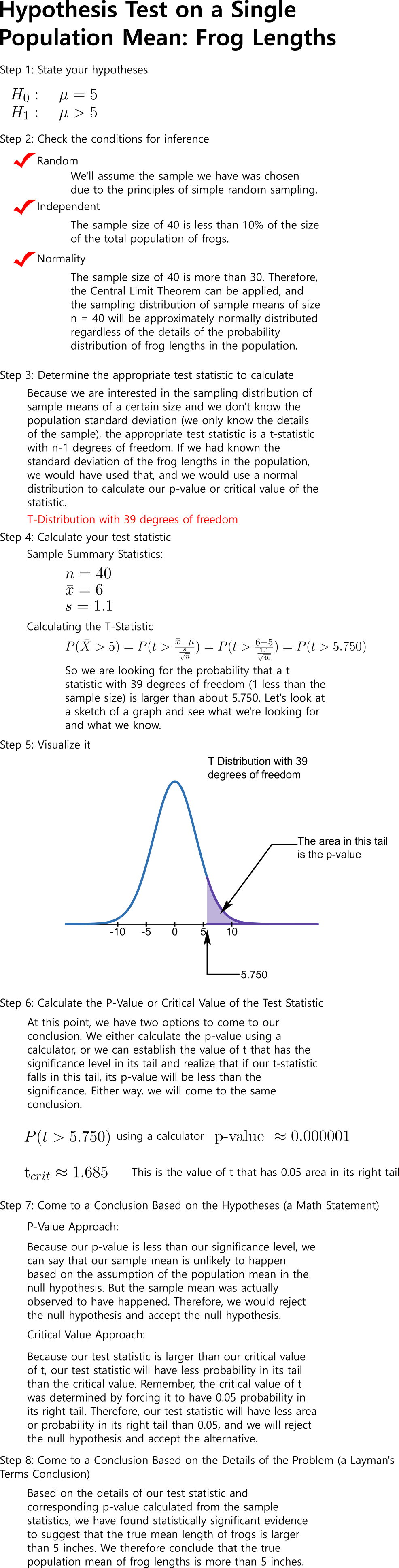
So as you can see, our intuition was right. It turns out that the probability of getting a sample of size 40 with a mean 6 inches if the population mean of frog lengths was really only 5 inches is incredibly unlikely. How unlikely? That’s what our p-value tells us. But, remember that it depends on the variability of the data which we accounted for in our analysis. So using sampling distributions, we don’t have to guess at how likely or unlikely our data is based on the assumption of the population distribution. We can actually calculate it and therefore defend our conclusion.
Now this was an extensive discussion for a hypothesis test on a single population’s mean. All other hypothesis tests have the same sets of steps. The details of the conditions that have to be met, the distribution of the test statistic that you use, and some of the other steps may be a little different, but the flow of the logic and how you support you final conclusion are all based on the same idea. If you understand what a hypothesis test is really well one time, you can apply that logic to any other hypothesis test. The videos at the end of this lesson delve into other examples of hypothesis testing.


Leave a Reply