ericktutoring

Tag: philosophy

Sequences and Series: The Basics

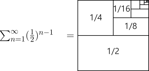
What are Sequences and Series?

Sequences and series are topics covered near the end of a Calculus 2 class, but show up in all kinds of situations. Let’s discuss what these two concepts mean in a little bit of detail. A sequence is just an ordered list of numbers or terms. For instance, the following would be considered a sequence:

$\{1, 3, 5, 7, 9, 11, 13 \}$

In this sequence, the numbers in the sequence can be thought of as the output from a function, or the y-values. So what are the x-values? The x-values are the positions that the numbers take in the sequence. Looking back at the previous sequence, we can see that the 3rd number in the sequence is a 5. Therefore, you can think of this sequence as a function where it takes an input of 3 and produces an output of 5. The “position” we keep referring to is called an “index”.

Many sequences of interest can be written as a mathematical expression that illustrates how the index becomes the sequence value (exactly how most functions are written as mathematical equations that detail how each input in the domain becomes each output in the range). Let’s try to come up with the mathematical relationship that maps the indices to the terms in the sequence. If you notice, the terms in the sequence are just the odd integers from 1 up to 13. So what mathematical expression, if any, would turn 1 into 1, 2 into 3, 3 into 5, 4 into 7, and so on? Well first, let’s pretend that the numbers in the sequence were the even integers. How would we turn 1 into 2, 2 into 4, 3 into 6, and so on? That’s a much easier relationship. You just double the index, and now you have the even integers. So how do we get the odd integers? Easy, just subtract 1 after you double the indices. This can be summarized in the following equation:

$a_n = \{2n-1\}_{n=1}^{7}$

This means that we have a sequence with the formula inside the curly brackets with an index that starts at 1 and ends at 7. In other words, we have 7 terms in our sequence (1 through 7) and to get the number at the n^th index, you do the math inside the curly brackets. So how is this different from the function:

$f(x) = 2x – 1 \quad 1 \leq x \leq 7$

These look like they’re saying the same thing to me. Well, they’re not because it really comes down to the difference between the variable $n$ and the variable $x$ . Remember that the variable n represents the index. That means that it represents the place that the associated term takes in the ordered list of terms that make up the series. So the “domain” of a series can only ever be integers since they represent the position of the terms in the list. However, the variable x is assumed to be a continuous variable. Therefore, in the previous function, x can take any value from 1 to 7 including decimals and fractions and anything else you can think of. This would be clear from the graphs of the sequence vs. the corresponding function. The graph of the sequence would only consist of 7 points. There would be a point at (1, 1), (2, 3), (3, 5), and so on, but there would be nothing in between since there is no index or position in the list of numbers between 1 and 2 or 2 and 3 and so on. The graph of the corresponding function would consist of a solid curve (a line in this case) defined by the function $2x-1$ . But the curve would go through all the same points defined by the sequence if you think of the values of n as x-values and the sequence values as y-values. So in a lot of ways, sequences are like functions with the condition that the input variable can only be integers within a certain domain.

In a Calculus 2 class, you’ll be mostly interested in sequences that have infinite terms. So the ordered list of terms or numbers is infinitely long without end. In this situation, we would be interested to know if the sequence converges or diverges. In this context, that just means that the numbers or terms that form the sequence start to approach a single value or term as you proceed infinitely down the list of numbers. This should sound familiar. I’m describing a limit. Therefore, to determine whether or not a sequence $a_n$ converges, we just need to find the value of the following limit:

$\lim_{n \rightarrow \infty} a_n$

If this limit has a value, then the sequence converges. If this limit does not have a value (either because the value of the limit is $\pm \infty$ or the values in the limit do not go to a specific number as you go infinitely far down the positions in the sequence), we would say that the sequence diverges. That’s all you have to know when it comes to sequences. Whether or not they converge or diverge only comes down to the value of the limit and whether or not it exists. One concept or idea that you will need to brush up on is how to evaluate limits at infinity.

So we’ve been talking a lot about sequences so far and haven’t discussed anything about series yet. Are they the same thing? No. They’re similar, but they’re not the same. In fact, a series is just the sum of the terms in a sequence. That’s it. If you have a sequence and you add all the terms in the sequence together, you now have the corresponding series. With series, we’ll primarily be interested in those series that come from the summation of an infinite sequence. To determine whether a series converges or diverges, we’ll need to determine whether the sum of an infinite number of things adds up to a single number or if it does not. This is a much more difficult question to try and answer. There are many different convergence and divergence tests that are designed to determine whether or not a series converges. Just like solving an integral requires knowing certain integration techniques and when to use them, determining whether a series converges or not requires knowing certain convergence and divergence tests and when to use them.

Some Basic Types of Series and Convergence/Divergence Tests

For the rest of this blog post, we’ll look at some qualities and behaviors of series, discuss some common series you should know, and finally introduce some of the simplest convergence and divergence tests for series. First, let’s dive into the apparent contradiction of an infinite series. For an infinite series, we’re interested in whether it converges or not. This means we are interested in whether you get a specific number when you add up an infinite number of numbers. Why do we even need convergence and divergence tests for series? It seems like they would never converge, right? How in the world can you add up an infinite number of numbers and not get infinity or negative infinity? The answer is if the terms eventually become zero or if they shrink towards zero at a certain rate as you progress down the sequence of numbers your adding, the sum can be a finite amount. You’ve actually seen this before. In the context of the definite integral, we saw that you can add up an infinite number of things (rectangular slices of the region bounded by a curve) as long as the terms get smaller at a certain rate with the number of things that you’re adding.

N^th Term Divergence Test

So that actually brings us to our first type of convergence/divergence test. It is called the N^th Term Test for Divergence. This test is basically mathematically equivalent to the only convergence/divergence test we needed for sequences:

$\lim_{n \rightarrow \infty} a_n$

For a sequence, the result of this limit tells us whether or not the terms in the sequence eventually tend toward a certain value or not as you progress infinitely far down the ordered list of terms. So how is this useful information for the infinite sum $\sum_{n=1}^{\infty} a_n$ ? Well, what this limit literally tells us is what the numbers in the list of numbers we’re adding together start to become as you go infinitely far down the list. What would these numbers have to eventually converge to if the infinite sum has even a chance of converging? The answer is 0. If the infinite sum of numbers has even the slightest chance of adding up to a finite amount, the terms in the sequence would eventually have to start to become infinitesimally close to 0. That’s the basic idea of the Nth Term Test for Divergence. So what we can conclude is that if the numbers in the infinite sequence that we’re adding together to form the infinite series (or sum) DO NOT eventually get infinitesimally close to 0, then the series has no chance of converging, and we can conclude that it diverges.

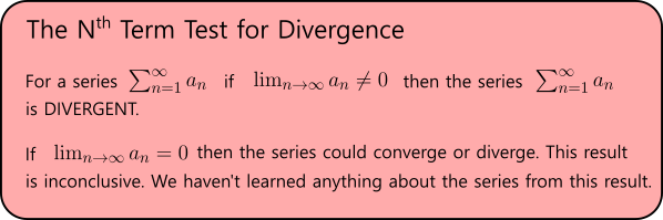
Let’s look at what this Nth Term Test for Divergence is saying. Basically, it says that if the terms in the series do not eventually get indistinguishably close to zero, we can conclude that the series diverges. This should make perfect sense. What would happen if you added up an infinitely long list of numbers (an infinite sequence), and the numbers in the list don’t become super close to 0? Then the sum would either add up to infinity or negative infinity, or the sum would not add up to anything specific. Either way, the series would not sum to a single finite amount. But let’s look at the other result. What if the numbers in the sequence your summing to form the series do eventually get down infinitesimally close to 0? Well that sounds like the series would have to converge since you’re eventually adding 0 over and over again forever, right? At this point our simple logic is starting to break down. We’ll prove this later, but for right now, just take my word for it that just because the numbers do eventually get down infinitesimally close to 0, that may not be enough. If the terms do eventually get down infinitesimally close to 0, you need to analyze the rate at which they get down close to 0. If you want to understand how it is possible for a series with terms whose limit as n approaches infinity is zero to not converge, think of a corresponding improper integral with an infinite upper bound for the limit of integration. If the function your integrating eventually gets down infinitesimally close to 0, that means the height of the region whose area you’re finding with that integral is getting infinitesimally close to 0. Doesn’t that mean that the area has to be a finite amount? Well, calculate the following integral, and you’ll see that just because the function that defines the height of the region eventually becomes infinitesimally small, that doesn’t mean that the area of the bounded region converges:

$A= \int_{1}^{\infty} \frac{1}{x} \ \ dx$

In fact, if you can make the connection between infinite series and their corresponding improper integrals, you can better understand the next convergence/divergence test that you’ll probably learn in class called The Integral Test. We’ll talk about that in a later post.

Partial Sums

One way that we can determine whether a series converges or diverges is to convert it to a sequence of partial sums and investigate if that sequence converges or not. Partial sums are just a running total of the total sum as you add one term to the previous term. These are generally denoted as $s_n$ .

For the series

$\sum_{n=1}^{\infty} a_n$

We can show the partial sums as

$s_m = \sum_{n=1}^{m} a_n$

$s_m = a_1+a_2+a_3+a_4+ \dots +a_{m-1}+a_m$

In other words, the m^th partial sum $s_m$ is just the first “m” terms in the corresponding sequence added together. Let’s look at some of the math involved and how these partial sums reveal what’s going on with the infinite series. First, we should notice that the m+1^st partial sum $s_{m+1}$ is just the m^th partial sum $s_m$ plus the next term in the series $a_{m+1}$ .

$s_m = a_1+a_2+a_3+a_4+ \dots +a_{m-1}+a_m$

$s_{m+1} = a_1+a_2+a_3+a_4+ \dots +a_{m-1}+a_m+a_{m+1}$

$s_{m+1}-s_m = a_{m+1}$

$s_{m+1}=s_m + a_{m+1}$

So if we define a new sequence $\{ s_m \}$ where $s_m = \sum_{n=1}^{m} a_n$ or the m^th partial sum, the result of the convergence of this SEQUENCE of partial sums would be the result of the convergence of the corresponding infinite SERIES. So if we can come up with a formula for the m^th partial sum of a series, we could then determine the convergence or divergence of that corresponding sequence of partial sums and determine if the series converges or diverges. This brings us to two specific types of series for which you can determine a formula for the corresponding sequence of partial sums.

Telescoping Series

A telescoping series is a series in which most of the terms end up adding up to zero such that a large sum can really be calculated by adding only a small number of the total terms. Something that “telescopes” in real life is like the hydraulic cylinder in the following picture. It is composed of concentric tubes that can extend out to form one long tube, or these concentric tubes can be collapsed down to a smaller form:

If I could rename what a Telescoping Series is, I may rename it to a Collapsible Series because that’s really the behavior these types of series exhibit that make them interesting. Let’s see what this type of series looks like in action. Take the following series:

$\sum_{n=1}^{\infty}\left( \frac{1}{n} – \frac{1}{n+1} \right)$

Let’s now take a look at the partial sums:

$s_1 = \sum_{n=1}^{1}\left( \frac{1}{n} – \frac{1}{n+1} \right) = \frac{1}{1} – \frac{1}{2}$

$s_2 = \sum_{n=1}^{2}\left( \frac{1}{n} – \frac{1}{n+1} \right) = s_1 + \frac{1}{2} – \frac{1}{3}= \frac{1}{1} – \frac{1}{3}$

$s_3 = \sum_{n=1}^{3}\left( \frac{1}{n} – \frac{1}{n+1} \right) = s_2 + \frac{1}{3} – \frac{1}{4}= \frac{1}{1} – \frac{1}{4}$

$s_4 = \sum_{n=1}^{4}\left( \frac{1}{n} – \frac{1}{n+1} \right) = s_3 + \frac{1}{4} – \frac{1}{5}= \frac{1}{1} – \frac{1}{5}$

Notice a pattern yet? What if I asked you to write out the formula for the m^th partial sum $s_m$ ?

$s_m = \sum_{n=1}^{m}\left( \frac{1}{n} – \frac{1}{n+1} \right) = \frac{1}{1} – \frac{1}{m+1}$

The pattern is that there is always the first positive term that remains and there is one negative term that remains at the end. So now we have a formula to find the m^th partial sum. What can we do with that? We can determine the convergence of the infinite sequence of partial sums to determine the convergence of the corresponding series. So now we’re back to analyzing a sequence. We just have to investigate the limit as m approaches infinity:

$\lim_{m \rightarrow \infty} \frac{1}{1}-\frac{1}{m+1} = 1-0 =1$

Therefore, we now know that this telescopic series converges to 1 because the sequence of partial sums converges to 1.

Geometric Series

A geometric series is another type of series where we’re able to come up with a formula for the sequence of partial sums. But what even is a geometric series? Geometric series are related to exponential functions. In a geometric series, the next term that you add to the previous partial sum to get the new partial sum is always the same number multiplied to the previous term:

$a_{n+1} = r \cdot a_n$

This multiplier is called the common ratio “r”. This is similar to an exponential function where every time you increase x by 1, the new function value is the the same number times the function value before it:

$f(x) = r^x$

$f(x+1) = r^{(x+1)} = r^x \cdot r^1 = r \cdot r^x$

Therefore:

$f(x+1) = r \cdot f(x)$

Because of this behavior, a geometric series can be written in this general form:

$\sum_{n=1}^{\infty}a_1 \cdot r^{n-1}$

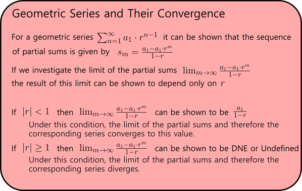
From this relationship, the following properties can be derived for a geometric series. Hopefully, proofs for these properties were offered in class or in your notes. If not, we can go through them in a later post. But for now, take my word that the following is true:

So now let’s see this in action with an example of a geometric series. Let’s take the series:

$\sum_{n=1}^{\infty} 15\cdot \frac{4^n}{12^{n+3}}$

Now this doesn’t look like the exact form of a geometric series that we discussed before ( $\sum_{n=1}^{\infty}a_1 \cdot r^{n-1}$ ). However, if every next term in the sequence of numbers is the same multiplier of the previous term, then it is geometric no matter what the formula looks like. Let’s see how we can determine this.

$r = \frac{a_{n+1}}{a_n}=\frac{15\cdot \frac{4^{n+1}}{12^{(n+1)+3}}}{15\cdot \frac{4^n}{12^{n+3}}}= \frac{15 \cdot 4^{n+1} \cdot 12^{n+3}}{15 \cdot 4^n \cdot 12^{n+4}} = \frac{4}{12} = \frac{1}{3}$

Now do you see that we took an arbitrary term $a_{n+1}$ and divided it by the previous term $a_n$ without specifying what n is, and it still ended up where all the n’s divided out? Because we found that the value of any term divided by the previous term without specifying which specific term we’re referring to reduces to a constant ratio ( $\frac{1}{3}$ in this case), this proves that the series is geometric. So not only do we now know that this series is a geometric series, we can also determine if it is convergent or not because we determined the value of the common ratio in the process of determining whether or not it was geometric, and the convergence or divergence of a geometric series only depends on the value of this common ratio. So we just ask ourselves, is the absolute value of the common ratio less than 1 or is it greater than or equal to 1? Since $\frac{1}{3}$ is less than 1, we know that this geometric series will converge.

But we can do better than that. Remember, for a geometric series (like a telescoping series), we actually have a formula for the partial sums. We therefore know that because the series converges, it will specifically converge to $\frac{a_1}{1-r}$ . We know $r$ , but do we know $a_1$ ? Well, if you try to compare our geometric series with the formula for a geometric series that lists out $a_1$ , you’d be tempted to say that $a_1$ is probably 15, right? Well it’s actually not. And the reason why is because what $a_1$ really represents is the first term in the geometric series. In our geometric series, I can tell you that the first term is not 15. So what is it? We can figure it out by just substituting 1 in for n and that will produce the value of $a_1$ .

$a_1 = 15\cdot \frac{4^1}{12^{1+3}} = 15 \cdot \frac{4}{12 \cdot 12^3} = \frac{15}{3 \cdot 12^3} = \frac{5}{1728}$

Therefore, the actual sum of the series $\sum_{n=1}^{\infty} 15\cdot \frac{4^n}{12^{n+3}}$ is $\frac{\frac{5}{1728}}{1-\frac{1}{3}}$ which simplifies to $\frac{5}{1152}$ .

Summary

In summary, a sequence is an ordered list of numbers which you can think of like a function. What you input is the position of the number in the list, and what you get out of the function is the number that goes in that position. To determine whether or not a sequence converges, there is only one test. You determine the limit of the function that defines the sequence as the value of the index goes to infinity. If this limit exists, the sequence converges to that value. If the limit does not exist, the sequence diverges.

Series are much more complicated. A series is the sum of a sequence. A series converges if the sum of the infinite sequence it represents is a single finite amount. If the sum of the infinite sequence is not a single finite amount (either because it’s not a single determinant amount, or if it’s not finite), then the series diverges. But to prove if an infinite sum converges or not requires you to be much more clever. There are lots of different convergence and divergence tests for series. The most basic one we talked about in this post is the N^th Term Test for Divergence which operates on a simple principle. If the terms in the sequence that form the series never approach 0, then the sum cannot be a specific finite amount. However, if the terms in the sequence that form the series do approach 0, that leads to an inconclusive result. The series could converge or diverge still.

By looking at the sequence of partial sums, we can determine if the infinite sum is approaching a single value or not. We discussed two types of series for which you can determine a formula for their partial sums: a telescoping series and a geometric series. By understanding what these two series are and how they behave, we can easily determine whether or not they converge and what they converge too. This is a very important distinction between these types of series and most of the other series that you come across. For most series, you will not be able to determine what they converge to specifically. You will only be able to determine whether or not the series converges at all.

November 1, 2026
Your Best Friend: The Unit Circle Part 1
What is The Unit Circle?

The unit circle is a clever visual tool that can be used to analyze various aspects of trigonometry. First of all, it’s a circle. And while you may be most familiar with thinking of trigonometric functions in the context of right triangles, they can actually be thought of as parts of a circle. One of the limitations of thinking of trigonometric ratios solely from the perspective of right triangles is that the angles on a right triangle are restricted to be between zero and ninety degrees (0 to pi radians). However, the trigonometric functions are defined well outside this domain. Thinking of the trigonometric functions in the context of a circle allows you to analyze trigonometric relationships for any angle. Also, the definitions of the trigonometric functions in the context of right triangles naturally extends to their analysis as being part of a circle. In other words, you don’t have to relearn anything you know about trigonometry and right triangles to make sense of the unit circle approach to trigonometry. You just have to be able to expand your view to accommodate more possibilities. Everything you know about trigonometry using right triangles is still true on the unit circle. The unit circle just extends this analysis even further. What we’ll talk about in this article is specifically how to map your knowledge of trigonometry using right triangles onto the unit circle in order to take advantage of its greater capabilities in understanding trigonometry.

The “unit” part of the unit circle has a specific meaning. Typically, any time you hear or see the word “unit” in the context of mathematics, it means 1. For instance, in more advanced math using vectors, you’ll hear the term “unit vector” which means a vector with a length of 1. So what about the unit circle is 1? Its radius is 1. As we’ll see when we’re mapping our right triangles onto the unit circle, the hypotenuses of these right triangles will be the same length of the radius of the circle.

To analyze the trigonometry on a unit circle, the x and y coordinates of the points on (and sometimes off) of the circle are important. Therefore, this unit circle doesn’t mean anything without a relevant coordinate system. The location of the unit circle in the x-y plane is such that its center is at the origin. So to summarize, the unit circle is a circle with radius 1 centered at the origin of the x-y plane.

How does the unit circle work in explaining trigonometric functions?

The basic principles allowing the unit circle to be used for analysis of trigonometric functions are few and simple. Here they are:
1. Angles are measured from the positive x-axis. Counter-clockwise rotations are positive angle changes. Clockwise rotations are negative angle changes.
2. The x-value of a point on the circle is equivalent to cosine of the angle formed by the radius that extends out to that point and the positive x-axis
3. The y-value of a point of the circle is equivalent to sine of the angle formed by the radius that extends out to that point and the positive x-axis
This can be shown with a simple diagram:

From these simple basic principles (along with all the analytical trigonometry you know), the unit circle can be used to analyze complicated problems involving trigonometry.

Basic Trends that Emerge from the Unit Circle

Because the x values of the points on the unit circle are the values of cosine of the corresponding angle and the y values of the points on the circle are the values of sine of the corresponding angle, we can see pretty easily the quadrants in which cosine and sine are negative and positive. This is summarized in the following figure:

This all comes from the idea that $\cos{\theta}$ is x and $\sin{\theta}$ is y. In the first quadrant, $\cos{\theta}$ and $\sin{\theta}$ are both positive. Why? Because x and y are both positive in the first quadrant. In the second quadrant, $\cos{\theta}$ is negative and $\sin{\theta}$ is positive. Why? Because x is negative and y is positive in the second quadrant.

Knowing the signs of $\sin{\theta}$ and $\cos{\theta}$ at different angles allows you to immediately determine the signs of the other 4 trigonometric functions for that value of $\theta$ . For instance, we know from the reciprocal identities that $\tan{\theta} = \frac{\sin{\theta}}{\cos{\theta}}$ . Therefore, we know that any angle where $\sin{\theta}$ and $\cos{\theta}$ have the same sign, $\tan{\theta}$ will be positive (the first and third quadrants). And any angle where signs of $\sin{\theta}$ and $\cos{\theta}$ have different signs, $\tan{\theta}$ will be negative (second and fourth quadrants).

Some other trends that we should notice is how the two functions $\sin{\theta}$ and $\cos{\theta}$ change as the angle $\theta$ changes. We can determine this at a general level by just looking at the unit circle. Let’s start by looking at a specific angle. Let’s look at $\theta = 0 ^ {\circ} \: \text{or} \: 0 \, \text{radians}$ . This corresponds to the point on the following diagram of the unit circle.

Now we need to just ask ourselves, as $\theta$ increases (we rotate counterclockwise from this point), what happens to the x and y values on the circle? Well, you should notice that the x value doesn’t change that much when you change the value of $\theta$ a little bit. However, the value of y changes a lot when you change the value of $\theta$ a little bit. So around the value $0^{\circ} \, \text{or} \, 0 \, \text{radians}$ , $\cos{\theta}$ changes very slowly and $\sin{\theta}$ changes relatively quickly.

But how are the functions changing when it comes to their values? Well we can look at the unit circle again and determine the answer. As we rotate around circle counterclockwise, the value of $\cos{\theta}$ decreases from its maximum value of 1 (the x value of the points on the unit circle decrease from the maximum value of 1), and the value of $\sin{\theta}$ increases from 0 (the y value of the points on the unit circle increase from their value of 0). Once we hit the angle of $\frac{\pi}{2} \, \text{or} \, 90^\circ$ , the trend changes a little bit. Now we’re at the top of the circle and the value of $\cos{\theta}$ or x is changing fast (we’re basically moving horizontally for a moment at the top of the circle) and the value of $\sin{\theta}$ or y is changing slowly (again, because we’re basically moving horizontally, the y-values don’t change very quickly). Also, let’s again look at how their values are actually changing. $\cos{\theta}$ is still decreasing (as you rotate around the counterclockwise direction at the top of the circle, the x-values are still decreasing) and it actually becomes negative, and $\sin{\theta}$ actually starts decreasing as well from a maximum value of 1 (the y-values are at their largest, and start to decrease from 1 as you continue to rotate around the circle). We can continue to analyze these trends around the circle. This will be very useful when we look at how to determine the wave graphs of $\sin{\theta} \, \text{and} \, \cos{\theta}$ later.

What specific values are you supposed to know on the unit circle?

So this is the main reason you need to know the unit circle. Other than the trends and behavior that the unit circle reveals about trigonometric functions, there are specific values of $\cos{\theta}$ and $\sin{\theta}$ (x and y) that you need to know for specific angles. Here is the full annotated unit circle with all of the values you need to know. At first, it looks daunting. But we’ll see in a moment that you only really need to know a few of these points and angles in order to be able to figure out the rest due to some of the symmetries that exist in circles.

So these are all of the angles and points you need to know on the unit circle. It seems pretty daunting at first, but there are actually quite a few patterns we can observe. In fact, you only need to know the angles and ordered pairs in the first quadrant. From there, you can take advantage of all the symmetries of the circle to fully annotate all four quadrants. So let’s just look in depth at the first quadrant. Which angles do we need to know? From the diagram that includes the angles, we can see that we need to know the values of $\sin{\theta}$ and $\cos{\theta}$ for $0^\circ$ , $30^\circ$ , $45^\circ$ , $60^\circ$ , and $90^\circ$ . You just need to memorize the angles. One way to remember these angles is to realize they account for the $90^\circ$ that forms the first quadrant broken up into thirds ( $0^\circ$ , $30^\circ$ , $60^\circ$ , and $90^\circ$ ) and halves ( $0^\circ$ , $45^\circ$ , and $90^\circ$ ).

Now how do we remember the values of x and y (and therefore cosine and sine) for these angle values? There is actually a nice pattern that emerges in the numbers. Don’t ask me why this pattern exists. I have no idea why this interesting pattern emerges. It’s just something I’ve noticed that can help you remember the values you need to know in the first quadrant. First think of all of the values of x and y on the circle as square root of something divided by 2. You can see what I mean in the following figure:

Now, let’s start filling these in. Inside every square root goes either a 0, 1, 2, 3, or 4. Let’s start with the point at angle 0 radians (the point that’s on the x-axis). What goes inside the square roots for the x and y? In the x-value, we’ll need to put a 4 inside the square root, and for the y-value, we’ll need to put a 0 inside the square root. But how does this make sense? Well, what is the x-value at that point? It should be 1. Remember, this is the unit circle centered at the origin with a radius of 1. Therefore, that point that is one full radius in the x-direction from the center would have an x-value of 1 plus the x-value of the center of the circle. Because the x-value of the center of the circle is 0, the x-value of this point is 1. So why did we put in 4? It’s because that’s inside a square root. The square root of 4 is 2, and 2 divided by 2 gives us the ultimate x-value of 1 that we know that needs to be. So that’s why the x-value of this point is $\frac{\sqrt{4}}{2}$ . Now what about the y-value? Well, that’s obviously 0 at this point. It’s the same y-value as the center of the circle because we didn’t move up or down from the center. We just moved left or right. So what do we need to put inside the square root to make the total value 0? That would be 0 because $\frac{\sqrt{0}}{2} = 0$ . So let’s put these points in the first quadrant of the unit circle.

So now that we have the “first point” set, the pattern that emerges is that we just lower the value of the number inside the square root for the x-values by 1 at each new point as we rotate counter clockwise, and we just raise the value of the number inside the square root for the y-values by 1 at each new point as we rotate counter clockwise.

Now let’s just simplify these values:

So now we have the entire first quadrant filled out. How do we get the x and y values ( $\cos{\theta} \ \text{and} \ \sin{\theta}$ ) for all the other points on the circle? Well, we can take advantage of the symmetry of the circle and notice that all of the other points are just transformations of the points we already have. Let’s take a look at the second quadrant. Theses are all the same x and y values, but the x values are negative because it’s like we’ve flipped the second quadrant across the y-axis without moving up or down. That causes the x-values of the points to be the opposite sign.

Now we have all of the points in the first and second quadrant. How do we get the rest of the points in the third and fourth quadrant? Well we can notice that due to the symmetry of the circle, the points on the bottom half (the third and fourth quadrants) are reflections of the points in the top half across the x-axis. This transformation just keeps all the x-values the same, but negates all of the y-values.

Now we have the full unit circle filled out with all of the important points labeled. This was all based on a simple pattern that we notice in the first quadrant and the fact that the other quadrants are the same points as the first quadrant just reflected across the different axes. We can now use this information to answer questions and solve problems involving trigonometry. We’ll look at that in the next blog post.

Summary

In summary, the unit circle is a useful tool to visualize the trigonometric functions $\sin{\theta}$ and $\cos{\theta}$ and their behaviors as the angle $\theta$ changes. The unit circle is a circle centered at the origin with a radius of 1. In this context, the angle $\theta$ is defined as the angle created from an initial side on the positive x-axis where positive values of $\theta$ are created by rotating counter clockwise, and negative values are created by rotating clockwise from the positive x-axis. On the unit circle, the x-coordinate is $\cos{\theta}$ and the y-coordinate is $\sin{\theta}$ . Taking advantage of various symmetries of the circle, we can transpose and transform points around to find the values of $\cos{\theta}$ and $\sin{\theta}$ for various angles.
October 29, 2026